Compression

Making data smaller

Compression depends on redundancy

Imagine you have a piece of paper with words written on it and you had to describe to someone else what to write on their own piece of paper to make a copy.

Which would be easier to describe: a piece of paper with 100 copies of the same word or a piece of paper with 100 words chosen at random?

Entropy

How much we can compress something is a measure of how much information is in the data.

Lots of data = not very compressible.

This is also said to have high entropy

Maximum entropy is complete randomness which can't be compressed at all.

"You should call it entropy, for two reasons. In the first place your uncertainty function has been used in statistical mechanics under that name, so it already has a name. In the second place, and more important, no one really knows what entropy really is, so in a debate you will always have the advantage."

John von Neumann's advice to Claude Shannon.

Two flavors of compression

Run Length Encoding

A simple form of lossless compression.

If the data contains many repeated values we can encode them by writing the value once and then a number that says how many times it is repeated.

AAAABBBBBC can be encoded as A4B5C1

There are lots of subtleties in how RLE is implemented in real life.

Huffman coding

Another form of lossless compression.

Requires some analysis of the data to find the frequencies with which different symbols occur.

A variable length encoding. The most frequently occurring symbol can be represented with a single bit while others take maybe even more bits than representing them directly.

Huffman coding tree

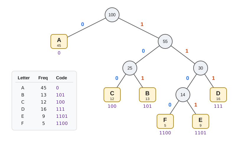
Image data

A trivial way to store images is as a sequence of numbers, each representing the red, green, or blue components of one pixel in the image.

Each of those numbers is essentially a numerator in an implicit fraction. If we use 16-bits per component that gives us a number from 0 to \(2^{16} - 1\), a.k.a. 65,535, so the denominator is \(2^{16} - 1\), giving us 65,536 gradations from 0.0 (none of that color) to 1.0 (all of that color).

Simple lossy compression

One simple way to compress image data is to simply use fewer bits per component.

For every 16-bit quantity, divide it by 256 (or right shift it by 8-bits) and store one byte instead of two.

Now we have only 256 gradations of each color but it will still be recognizably the same image.

Transform coding

Fancy math basis for better lossy compression.

Basically we can transform a series of N numbers into a series of coefficients picked so that if we multiply by a bunch of functions applied to the N positions [0, N) with those coefficients that when we add up the values returned by the functions multiplied by the coefficients at each position we get back the original numbers.

The transform is lossless

This step is itself lossless. It’s just representing the same set of numbers in a different way.

Basically we went from a list of N numbers to N coefficients and if the functions are known in advance we just need to store the coefficients.

Discrete Cosine Transform

If the functions we use in our transform are cosine functions cycling at different frequencies this is called a Discrete Cosine Transform or DCT.

After applying the DCT we can apply a slightly more sophisticated version of the simple lossy compression we described above to the coefficients and keep the same shape of the original data just with less precision.

Compressing the less-precise coefficients

The compression step is more sophisticated because it keeps more bits of the more important coefficients.

This means some of the less important coefficients get rounded to zero.

We can then use a combination of RLE and Huffman coding to represent the coefficients compactly.